T test in R
In this post, you will learn what a T Test is and how to perform it in R. First, you’ll see a simple function that lets you perform the test with just one line of code. Then, we will explore the intuition behind the test, building it step by step with data about the Titanic passengers. Enjoy the reading!
1. What is a T-Test?
A t-test is a statistical procedure used to check whether the difference between two groups is significant or just due to chance. In this post, we’ll look at data from Titanic passengers, dividing them into males and females. Suppose we want to test the hypothesis that men and women had the same average age. If our data shows that women were, on average, 2 years younger than men, we need to ask: is this a real difference, or could it have happened randomly? The t-test helps us answer this question.
2. Why is a T-Test important?
A t-test is important when we want to draw conclusions about a population based on a sample. For example, imagine we are studying the demographics of ship passengers at the beginning of the twentieth century and want to use the Titanic sample to generalize findings to a broader population of passengers.
Of course, such inferences may be biased, since Titanic passengers might not perfectly represent all ship passengers of that era. Nevertheless, the sample can still provide valuable insights, as long as the context of both the sample and the population is carefully considered and clearly explained.
3. The Titanic passengers
We are going to use the titanic R library to access data about Titanic passengers. Specifically, we will work with a subset of passengers contained in the titanic_train dataset. Below, you will find the code to load the data, calculate the mean and standard deviation of age for males and females, and show how many passengers are men and women.
library(titanic)
data('titanic_train')
df <- titanic_train %>%
    select(Sex, Age) %>%
    na.omit()

df %>% group_by(Sex) %>%
    summarize(mean(Age), sd(Age), n())
| Sex | mean(Age) | sd(Age) | n |
|---|---|---|---|
| female | 27.9 | 14.1 | 261 |
| male | 30.7 | 14.7 | 453 |
We can see that there is a difference of 2.8 years between the average age of men and women on the Titanic. Below, you can also check the distribution of ages.
ggplot()+
  geom_density(aes(x=df$Age, color = df$Sex), size = 0.7)+
  scale_color_discrete("")+
  xlab("Age")+
  ylab("Density")
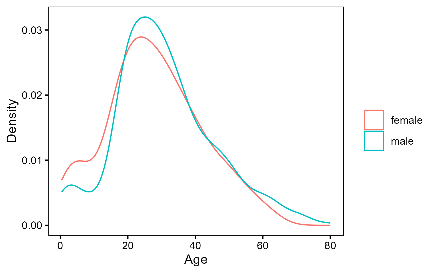
It seems indeed that the distributions are very similar. In this case, our best option is to carry a T Test out to see if they are really so similar.
4. T test in R
A T test can be performed in R in a very easy way. There is a function called t.test, whose first argument is a formula, in our case, we would like to know how age varies across different genders. Thomas Leeper wrote a very clear explanation about formulas in this page. Important for us is that the formula is composed by a dependent variable on the left (Age), followed by “~” and one or more independent variables on the right (Sex). The second argument is simply the dataframe with the data we want to test. This test assumes the two samples are independent and that age is approximately normally distributed, which we confirmed by the density plot above.
t.test(Age ~ Sex, data = df)
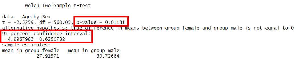
How to interpret these results?
- The p-value of 0.0118 means that if there were truly no difference in the average age between male and female passengers (i.e., if the null hypothesis were true), there would be only a 1.18% chance of observing a difference as large as the one we found or larger. Since this p-value is less than 0.05, we reject the null hypothesis at the 95% confidence level, suggesting that a real difference exists. However, if we had chosen a 99% confidence level, we would not reject the null hypothesis, because the p-value is greater than 0.01.
- Our confidence interval tells us that if we took many samples like the one we have, in 95% percent of the times, we would obtain a difference between averages between -0.62 and -5. This confidence interval does not include 0 and therefore we reject the null hypothesis and accept the hypothesis that there is a difference between the average age of men and women.
5. T test with Bootstrap
A T test with bootstrap is a good way of understanding the concepts needed to interpret the results of the T test above. Everything relies on the Central Limit Theorem according to which if I draw many samples of a population and calculate the mean of each sample, then the distribution of all these means will:
(i) follow a normal distribution;
(ii) the mean of the sample means will approximate the population mean;
(iii) the standard deviation of this distribution will be called standard error.
In our example, we have one sample of passengers. Imagine we could collect many of those samples. If we could do that, then the means of all samples would approximate the population parameter. Bootstrap is a technique to virtually create as many samples as we want from our unique sample. In our example, we have 712 ages after eliminating NAs. We could resample 712 observations from these values allowing them to repeat. That is the basic idea behind bootstrapping.
In order to do that procedure, we will create a function that will resample our data frame. The first line of code uses slice_sample to randomly select n rows of our dataframe allowing for the same row to be chosen more than one time. Note that n is the number of rows of the dataframe. After that, we use dplyr to calculate the mean by gender. Note that we are actually interested in the difference between the male mean and the female mean. That’s what the two last lines of code do.
diff_means <- function(data) {
    sample_df <- data %>% slice_sample(n = nrow(data), replace = TRUE)
    means <- sample_df %>%
        group_by(Sex) %>%
        summarize(mean_age = mean(Age, na.rm = TRUE))

    male_mean <- means %>% filter(Sex == "male")   %>% pull(mean_age)
    female_mean <- means %>% filter(Sex == "female") %>% pull(mean_age)
    return(male_mean - female_mean)
}
Now we can use the replicate function to execute our function for n times. For our purpose 1000 times is enough. Note that replicate works like a for loop. Before we do that, however, let us make a small adjustment so that we can also calculate our p-value. The p-value assumes the null hypothesis is true. Therefore, before resampling our data, let us make the difference between means be 0. For that, let us subtract the difference observed, 2.81, from the ages of all males.
df_null <- df %>%
    mutate(Age = ifelse(Sex=="male", Age-2.81, Age))

set.seed(1308)
diffs <- replicate(1000, diff_means(df_null))

sd(diffs)
mean(diffs)

ggplot()+
    geom_histogram(aes(x = diffs), color = "white", fill = "#2E3031")+
    geom_vline(xintercept = -2.8, color = "#A33F3F")+
    geom_vline(xintercept = 2.8, color = "#A33F3F")+
    scale_color_discrete("")+
    xlab("Age Differences (Null Hypothesis)")+
    ylab("Number of Individuals")+
    theme_bw()
Executing the commands above we get that the mean of the sampling distribution - as the distribution of the sample means is called - is approximately 0, as expected, and its standard deviation is 1.1.
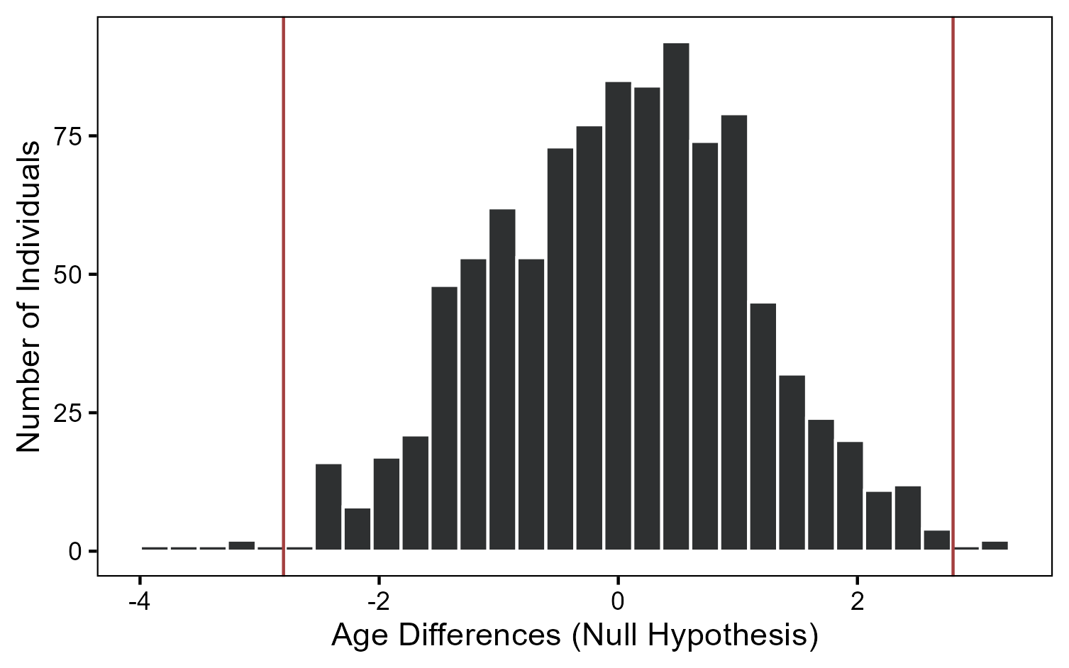
The histogram above shows us how the sample differences would look like if the null hypothesis were true. The red lines show the difference we observed in reality. Do you think it is likely to observe what we observed under the null hypothesis? It is actually not and you can calculate it with the code below:
sum(diffs>=2.81)/1000
sum(diffs<=-2.81)/1000
The code computes the number of samples whose means were more extrem than 2.8 (male age - female age) or -2.8 (female age - male age). This results in 9 samples out of 1.000, or 0.9%. This estimate is very close to the p-value found using the R function t.test. Again we can reject the null hypothesis and conclude that there is a difference between the average age of men and women.
In addition to helping us better understand the test, the bootstrap method has the advantage of not assuming that the age distribution follows a normal distribution. This is another benefit of using this approach.
Please, use the comments below if you did not understand a specific point of the test or if you have a suggestion to improve the test.
Comments
There are currently no comments on this article, be the first to add one below
Add a Comment
If you are looking for a response to your comment, either leave your email address or check back on this page periodically.