Chi-square distribution and test in R

Bruno Ponne ● 04 Dec 2023

• Advanced
• R
• 8 min

What you will learn

• Gain a clear understanding of the chi-square distribution;
• Master the concept of degrees of freedom through a practical example;
• Effectively perform a chi-square test to hypothesis testing;

Table of Contents

• 1. Data source
• 2. Why is the chi-square distribution useful for us?
• 3. Degrees of freedom in a chi-square test
• 4. How to estimate a contingency table under the null hypothesis?
• 5. Calculating chi-square in R
• 6. Conclusions

Greetings, humanists, social and data scientists!

Was there an association or relationship between gender and the verdicts in investigations in 18th-century London? If an inquest concerned a man, did this fact influence the final verdict of the investigation?

In this lesson we will answer these questions employing a chi-square test and the data explored in the lesson ‘How to Change Fonts in ggplot2 with Google Fonts’. You will learn what degrees of freedom are and how to harness the power of the chi-square distribution to infer relationships in historical London.

1. Data source

The dataset used in this lesson is made available by Sharon Howard. This dataset documents a range of Westminster inquests conducted between 1760 and 1799. Inquests were mostly investigations into deaths under circumstances that were sudden, unexplained, or suspicious. Please, check the lesson ‘How to Change Fonts in ggplot2 with Google Fonts’ for more information.

2. Why is the chi-square distribution useful for us?

The chi-square distribution is useful because it is the basis for testing the independence of two categorical variables. When we perform this test, the statistic we calculate follows a chi-square distribution. This enables us to determine the probability of observing a specific test statistic in our analytical sample under a certain hypothesis.

It’s not essential to know the function below, but understanding that the probability density function of a chi-square distribution follows this formula is beneficial. In the following steps we will write R code to generate a chi-square curve with n degrees of freedom and now you know that actually what R will compute is the function below with the n and x interval that you pass to the function. Note that f(0) = 0 and that \(\Gamma\) is the gamma function.

The area under this function gives us the probability of an interval of chi-squares happening. Fortunately, R has a function dchisq(x, df) that provides the chi-square density function. In the code below, we plot three chi-square distributions with 4, 8 and 16 degrees of freedom:

• to make it easier to plot the curves with color depending on the degrees of freedom, we create a data frame with three variables: x (from 0 to 50 in 0.1 steps); y (the result of the function f(n,x) above) and df (n degrees of freedom);
• in R, the chi-square density function is calculated with dchisq;
• color aesthetic is mapped to df (degrees of freedom) and to make sure ggplot uses discrete colors we transform degrees of freedom into a factor;
• scale_color_discrete is used to give a name to the legend and theme_coding_the_past() is our theme available here: ‘Climate data visualization with ggplot2’.

content_copy Copy

library(ggplot2)


x <- seq(0, 50, 0.1)

y1 <- dchisq(x, df = 4)
y2 <- dchisq(x, df = 8)
y3 <- dchisq(x, df = 16)

df1 <- data.frame(x = x, y = y1, df = 4)
df2 <- data.frame(x = x, y = y2, df = 8)
df3 <- data.frame(x = x, y = y3, df = 16)

df <- rbind(df1, df2, df3)

ggplot(data=df, aes(x = x, y = y, color = as.factor(df)))+
  geom_line(linewidth=1)+
  scale_color_discrete(name = "DF")+
  labs(y = "Density Function",
       x = "Chi-square")+
  theme_coding_the_past()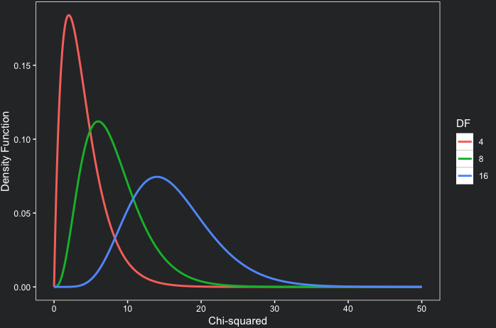

Note that as the degrees of freedom increase, the chi-square distribution increasingly resembles a normal distribution. With fewer degrees of freedom, the distribution exhibits more asymmetry.

3. Degrees of freedom in a chi-square test

As the plot above demonstrates, degrees of freedom are crucial as they determine the shape of our chi-square distribution. But what exactly are degrees of freedom?

Essentially, they represent the number of independent pieces of information allowed to vary in a system. For instance, in a contingency table, the degrees of freedom refer to the number of cells that can be varied, considering the total values observed in our sample. Is this concept a bit complex? I have created a video to illustrate this concept more clearly.

In a contingency table, degrees of freedom (DF) are calculated with the expression below, where nrows and ncolumns are the numbers of rows and columns, respectively.

4. How to estimate a contingency table under the null hypothesis?

Now that you’re familiar with the chi-square distribution and understand how to calculate degrees of freedom for a chi-square test, let’s explore how to derive our test statistic. Our aim is to determine if there’s an association between two categorical variables. Therefore, our alternative hypothesis (H1) posits that these two variables are dependent. Conversely, the null hypothesis (H0) suggests that the variables are independent.

In our case, we’re investigating the potential association between gender and verdict variables. To examine our contingency table, please run the following code. For an in-depth explanation of what this code accomplishes, refer to the lesson ‘How to Change Fonts in ggplot2 with Google Fonts’

H0: There is no association between gender and verdict.

H1: There is association between gender and verdict.

content_copy Copy

library(readr)
library(dplyr)
library(ggplot2)
library(showtext)

df <- read_tsv("wa_coroners_inquests_v1-1.tsv")

df_prep <- df %>% 
  filter(verdict != "-") %>% 
  mutate(verdict = recode(verdict, "suicide (delirious)" = "suicide",
                          "suicide (felo de se)" = "suicide",
                          "suicide (insane)" = "suicide"))

table_ver <- data.frame(table(df_prep$verdict))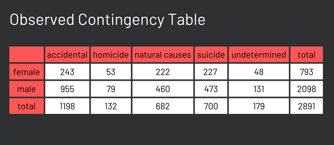

What would the above table appear like if the null hypothesis were true? In other words, if gender and verdict were truly independent, how would we calculate the expected values for each cell in that table? It’s important to remember that when events are independent, their probabilities are not influenced by each other. This principle is key to calculating the expected values in such a scenario.

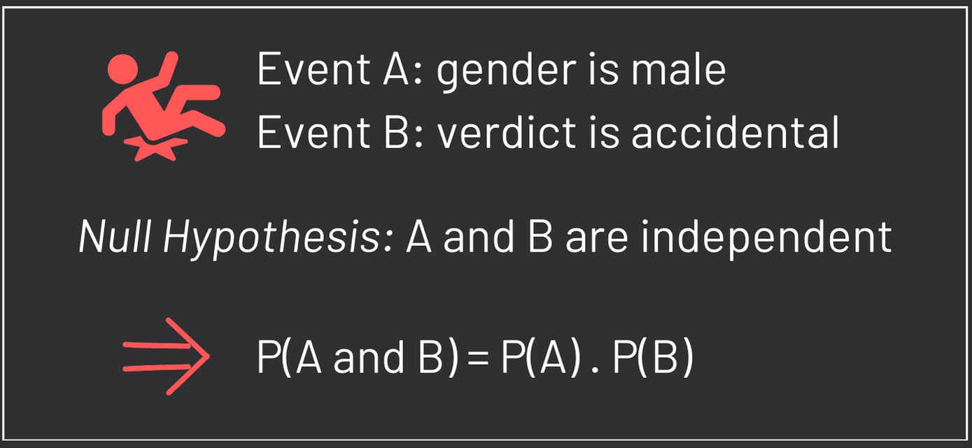
For instance, if we assume that the cause of death and gender are independent, we can calculate the probability of observing a case where a woman had an accidental death by multiplying the probability of the individual being a woman by the probability of an accidental death occurring. Once you’ve determined this probability, you can then multiply it by the total number of individuals in the sample to estimate the expected count for that specific cell in the table. This procedure is shown below.

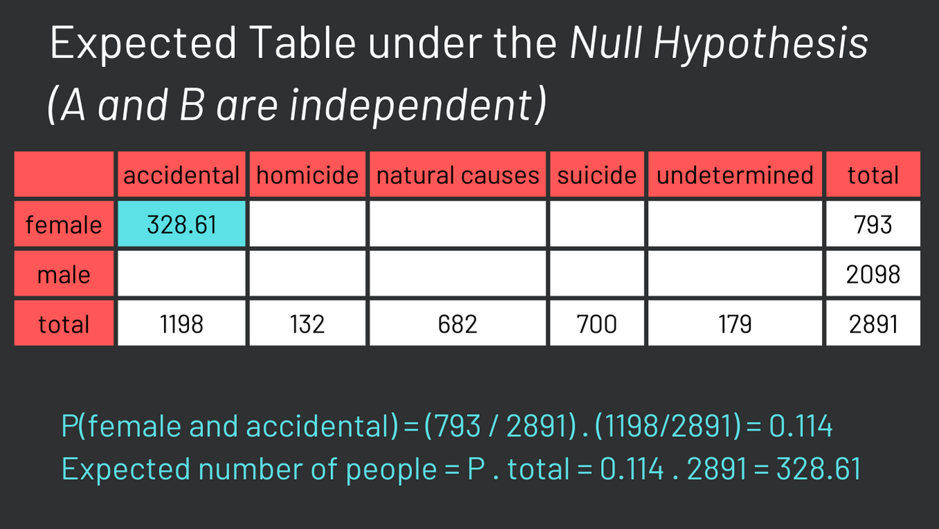
The calculation for the other cells in the table follows the same methodology. It’s worth noting that many textbooks present the following formula to calculate the expected values, which is based on the logic we’ve just discussed. In this formula, RT stands for row total; CT for column total; and TT for table total. You do not have to know this formula if you understood the underlying logic we explained earlier.

After you calculate all the expected values, it is time to calculate our test statistic.

5. Calculating chi-square in R

With both the observed and expected tables at hand, calculating the chi-square statistic becomes a straightforward process. For each cell, subtract the expected value (E) from the observed value (O), square this difference, and then divide by the expected value. Once you complete this calculation for every cell in the table, sum up these individual results. This sum is your chi-square statistic!

The next step is to determine how unusual this statistic is within the context of the chi-square distribution. It’s important to remember that this test statistic operates under the assumption that the null hypothesis is true. Therefore, the chi-square distribution will indicate the probability of encountering a chi-square statistic as large as, or larger than, the one you’ve calculated, under the assumption of the null hypothesis.

If you calculate it, you should find something around 59.3. We can plot a chi-square distribution with 4 degrees of freedom and estimate visually the probability of it. The code below does that and highlights the test statistic with a white dashed line. It is clear that a test statistic as large or larger than the one we obtained is extremely unlikely under the null hypothesis.

content_copy Copy

x <- seq(0, 70, 0.1)

y <- dchisq(x, df = 4)

df_4 <- data.frame(x = x, y = y, df = 4)

ggplot(data=df_4, aes(x = x, y = y))+
  geom_line(linewidth=1, color = "#C84848")+
  geom_vline(xintercept = 59.3, size = 0.4, color = "white", linetype = "dashed")+
  labs(y = "Density Function",
       x = "Chi-squared")+
  theme_coding_the_past()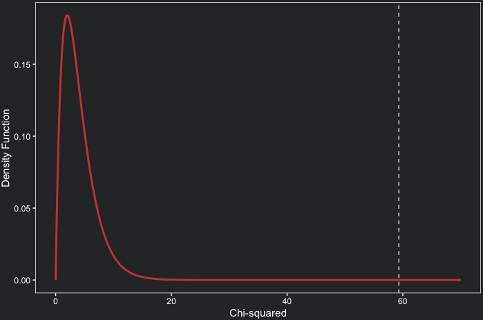

The good news is that the chisq.test function does all this work for us! In only one line of code you perform the test! With the code below you also get a numerical p-value to evaluate your hypotheses.

content_copy Copy

chi_test <- chisq.test(table(df_prep$verdict, df_prep$gender))

chi_test$statistic
chi_test$p.value
chi_test$expected

The result of chisq.test is stored in a list that I called chi_test. This list has several elements. Some of them are the chi-square statistic, the p-value and even the expected contingency table that we estimated above.

Now we can confirm analytically what we showed graphically above. The p-value tells us that the probability of observing a chi-square equal or larger than 59.3 is \(4.13 \times 10^{-12}\) under the null hypothesis. Our data is extremely unlikely under the null and therefore we can reject it. We can then accept the hypothesis that indeed gender and verdict are associated. Nevertheless, keep in mind that association does not mean causation.

These findings offer valuable insights into the distinct experiences of men and women in 18th-century London inquests. The results of our chi-square test suggest a relationship between the gender of the deceased and the outcome of an investigation. To further enrich our understanding of this statistical finding, a qualitative analysis could provide deeper context and detail. Your comments and questions are highly welcomed, so please feel free to share your thoughts and inquiries below!

6. Conclusions

• You can easily perform a chi-square test in R with the chisq.test function;
• Degrees of freedom play a crucial role in shaping the chi-square distribution, influencing the accuracy and reliability of our statistical inferences;
• The chi-square test reveals a significant association between gender and the verdicts of 18th-century London inquests, suggesting gender-based differences in investigation outcomes;