Understand TF-IDF in Python

Bruno Ponne ● 26 Apr 2023

• Medium
• Python
• 7 min

What you will learn

• Learn the concept behind TF-IDF;
• Be able to create a function that calculates TF-IDF;
• Learn to interpret TF-IDF scores;
• Be comfortable with visualizing your results.

Table of Contents

• Introduction
• Data source
• Coding the past: identifying relevant words in historical documents
  • 1. TF-IDF formula
  • 2. TF-IDF calculation example
  • 3. Preprocessing text data in Python
  • 3. Calculating term frequencies for each document
  • 4. Calculating how many times a word appears in each document in the corpus
  • 5. TF-IDF calculation
  • 5. TF-IDF Visualization
• Conclusions

Introduction

“Changes are shifting outside the words.”

Annie Lennox

In the Text Data Visualization lesson we learned how to use term frequency to identify the most frequent words in a document. Nevertheless, this methodology focuses only on the prevalence of individual terms within a single document, neglecting the term’s occurrence across other documents within the corpus. As a countermeasure to this shortcoming, TF-IDF was introduced. TF-IDF stands for Term Frequency - Inverse Document Frequency. This numerical statistic serves to underscore the significance of a word within a document, relative to a broader collection or corpus. In this lesson, we’ll journey through the process of calculating TF-IDF scores and bring those abstract numbers to life through Python-based visualizations.

Data source

The data used in this lesson is available on the Oxford Text Archive website. It consists of a collection of pamphlets published between 1750 and 1776 by influential authors in the British colonies. These pieces depict the debate with England over constitutional rights, showing the colonists’ understanding of their contemporary events and the conditions that precipitated the American Revolution. In this lesson, we will focus on the pamphlets of Oxenbridge Thacher, James Otis, and James Mayhew. To know more about textual data sources, check this post: ‘Where to find and how to load historical data’

Coding the past: identifying relevant words in historical documents

1. TF-IDF formula

TF-IDF (Term Frequency-Inverse Document Frequency) is a numerical measure that indicates the importance of a word in a document taking into account how frequent the word is in other documents in the same corpus. It consists of multiplying the term frequency (TF) by the inverse document frequency (IDF), which is the logarithm of the total number of documents divided by the number of documents containing the term. The formula is as follows:

Where:

• \(w_{ij}\) is the tf-idf weight for word \(i\) in document \(j\);
• \(tf_{ij}\) is the number of times word \(i\) appears in document \(j\) divided by the total number of words in document \(j\);
• \(N\) is the total number of documents in the corpus;
• \(df_i\) is the number of documents in the corpus that contain word \(i\).

2. TF-IDF calculation example

Suppose you want to calculate the TF-IDF weight for the word “British”, which appears 5 times in a document containing 100 words. Given a corpus containing 4 documents, with 2 documents mentioning the word “British”, TF-IDF can be calculated by:

TF-IDF increases as the term frequency increases, but it decreases as the number of times the word appears in other documents in the corpus increases. Variations of the TF-IDF weighting scheme are often used by search engines as a central tool in scoring and ranking a document’s relevance given a user query.

3. Preprocessing text data in Python

We will be using the same functions from the lesson Visualizing Text Data to preprocess the text data. The functions are:

• load_text: loads the text from a txt file and returns a list of words;
• prepare_text: preprocesses the text by removing stopwords, removing words with less than 3 characters, and transforming all words to lower case;
• count_freq: counts the frequency of each word in the the document and returns a dataframe with the results.

content_copy Copy

from itertools import islice
from nltk.tokenize import word_tokenize
from nltk.corpus import stopwords
import pandas as pd
import matplotlib.pyplot as plt

def load_text(filename):
    my_text = list()
    with open(filename, encoding= "latin-1") as f:
        for line in islice(f, 0, None):
            my_text.append(line)
    my_text = [word_tokenize(sentence) for sentence in my_text]
    flat_list = [item for sublist in my_text for item in sublist]
    return flat_list

def prepare_text(list_of_words):
  #load stopwords:
  stops = stopwords.words('english')
  #transform all word characters to lower case:
  list_of_words = [word.lower() for word in list_of_words]
  #remove all words containing up to two characters:
  list_of_words = [word for word in list_of_words if len(word)>2]
  #remove stopwords:
  list_of_words = [word for word in list_of_words if word not in stops]
  return list_of_words

def count_freq(my_list):
    unique_words = []
    counts = []
    # create a list of unique words:
    for item in my_list:
      if item not in unique_words: 
        unique_words.append(item)
    # count the frequency of each word:
    for word in unique_words:
      count = 0
      for i in my_list:
        if word == i:
          count += 1
      counts.append(count)

    # create a dataframe with the words and their frequencies:

    df = pd.DataFrame({"word": unique_words, "count": counts})
    df.sort_values(by="count", inplace = True, ascending = False)
    df.reset_index(drop=True, inplace = True)
    return df

After loading the functions above, we can use them to preprocess the text data.

Now we load the manifests of three authors: Oxenbridge Thacher, James Otis, and James Mayhew. The results are stored in three lists called thacher, otis, and mayhew. After that, we preprocess the text data using the function prepare_text and count the frequency of each word in each document using the function count_freq. Results are stored in three dataframes called thacher_df, otis_df, and mayhew_df.

content_copy Copy

thacher = load_text('thacher-2021.txt')
otis = load_text('otis-2021.txt')
mayhew = load_text('mayhew2-2021.txt')

thacher_prepared = prepare_text(thacher)
otis_prepared = prepare_text(otis)
mayhew_prepared = prepare_text(mayhew)

thacher_df = count_freq(thacher_prepared)
otis_df = count_freq(otis_prepared)
mayhew_df = count_freq(mayhew_prepared)

3. Calculating term frequencies for each document

As we have seen, the first component to calculate the TF-IDF weight is the term frequency. We can calculate the term frequency for each document by dividing the number of times a word appears in the document by the total number of words in it.

content_copy Copy

thacher_df["TF"] = thacher_df["count"]/sum(thacher_df["count"])
otis_df["TF"] = otis_df["count"]/sum(otis_df["count"])
mayhew_df["TF"] = mayhew_df["count"]/sum(mayhew_df["count"])

4. Calculating how many times a word appears in each document in the corpus

To calculate \(df_i\), we will left join all our dataframes. Then, for each row (word) we will sum the number of times its term frequency is greater than zero. In other words, we will count in how many documents the word appears at least once. This value will vary from 1 to 3, since we have three documents in our corpus. This count can be made with the pandas method ne() that checks if the values in the columns specified are not equal (ne) to zero. The results are booleans that can be summed to get the number of documents in which the word appears.

content_copy Copy

#left join all dataframes:
thacher_otis = thacher_df[["word", "TF"]].merge(
    otis_df[["word", "TF"]], 
    on = "word", 
    how = "outer", 
    suffixes = ("_thacher", "_otis")).fillna(0)

thacher_otis_may = thacher_otis.merge(
    mayhew_df[["word", "TF"]],
    on = "word",
    how = "outer").fillna(0)

#rename TF column to TF_mayhew:
thacher_otis_may.rename(columns = {"TF": "TF_mayhew"}, inplace = True)

#count in how many documents each word appears:

thacher_otis_may["dfi"] = thacher_otis_may[["TF_thacher", "TF_otis", "TF_mayhew"]].ne(0).sum(axis=1)

5. TF-IDF calculation

Finally we have all elements to calculate the TF-IDF weight. Note that we will be using base 10 logarithms. To calculate the logarithm, we can use the library math and its method log10(). We use the apply() method to apply the logarithm to each row of dfi and then multiply it by the term frequency. The results are stored in three new columns called TF-IDF_thacher, TF-IDF_otis, and TF-IDF_mayhew. Note that dfi varies from 1 to 3, so when the word appears in all three documents, the logarithm element will be zero and consequently TF-IDF will be zero as well (\(log_{10} 1 = 0\)).

content_copy Copy

import math

thacher_otis_may["TF-IDF_thacher"] = thacher_otis_may["TF_thacher"] * thacher_otis_may["dfi"].apply(lambda x: math.log10(3/x))
thacher_otis_may["TF-IDF_otis"] = thacher_otis_may["TF_otis"] * thacher_otis_may["dfi"].apply(lambda x: math.log10(3/x))
thacher_otis_may["TF-IDF_mayhew"] = thacher_otis_may["TF_mayhew"] * thacher_otis_may["dfi"].apply(lambda x: math.log10(3/x))

5. TF-IDF Visualization

Now we can compare how the two methods define the 10 most important words in each document. Keep in mind that the term frequency does not account for the words in other documents of the corpus while TF-IDF does. TF logic is that the most important words are the ones that appear the most in the document. TF-IDF logic is that the most important words are the ones that appear the most in the document but not in the other documents of the corpus. TF-IDF is more sophisticated because it helps you to distinguish one document from the others.

content_copy Copy

#create 2 dataframes with the top 10 words for each method:

TF_IDF_thacher = thacher_otis_may[["word", "TF-IDF_thacher"]].sort_values(by = "TF-IDF_thacher", ascending = False).head(10)
TF_thacher = thacher_otis_may[["word", "TF_thacher"]].sort_values(by = "TF_thacher", ascending = False).head(10)

#plot:

fig, (ax1, ax2) = plt.subplots(1,2, figsize=(9, 3))

#barplot:
ax1.barh(TF_thacher["word"], TF_thacher["TF_thacher"], color = "#386cb0", edgecolor = "#386cb0")
ax2.barh(TF_IDF_thacher["word"], TF_IDF_thacher["TF-IDF_thacher"], color = "#f0027f", edgecolor = "#f0027f")

#title:
ax1.set_title("Thacher TF")
ax2.set_title("Thacher TF-IDF")
ax2.set_xticks([0, 0.001, 0.002, 0.003])

for ax in fig.axes:                             # iterate over ax1, ax2, ax3 to: 
    ax.invert_yaxis()                           # invert the y axis; 
    ax.grid(False)                              # eliminate grid;
    ax.title.set_color('white')                 # set title font color to white;
    ax.tick_params(axis='x', colors='white')    # set x axis font color to white;
    ax.tick_params(axis='y', colors='white')    # set y axis font color to white;
    ax.set_facecolor('#2E3031')                 # set ax background color to #2E3031;
    ax.spines["top"].set_visible(False)         # eliminate spines;
    ax.spines["right"].set_visible(False)
    ax.spines["left"].set_visible(False)
    ax.spines['bottom'].set_color('white')

#fig background color:
fig.patch.set_facecolor('#2E3031')
#layout:
fig.tight_layout()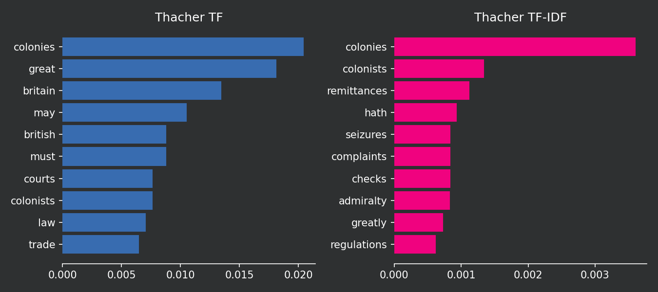

content_copy Copy

TF_IDF_otis = thacher_otis_may[["word", "TF-IDF_otis"]].sort_values(by = "TF-IDF_otis", ascending = False).head(10)
TF_otis = thacher_otis_may[["word", "TF_otis"]].sort_values(by = "TF_otis", ascending = False).head(10)

fig, (ax1, ax2) = plt.subplots(1,2, figsize=(9, 3))

# barplot:
ax1.barh(TF_otis["word"], TF_otis["TF_otis"], color = "#386cb0", edgecolor = "#386cb0")
ax2.barh(TF_IDF_otis["word"], TF_IDF_otis["TF-IDF_otis"], color = "#f0027f", edgecolor = "#f0027f")

# title:
ax1.set_title("Otis TF")
ax2.set_title("Otis TF-IDF")
ax2.set_xticks([0, 0.0005, 0.0010, 0.0015])

for ax in fig.axes:                             # iterate over ax1, ax2, ax3 to: 
    ax.invert_yaxis()                           # invert the y axis; 
    ax.grid(False)                              # eliminate grid;
    ax.title.set_color('white')                 # set title font color to white;
    ax.tick_params(axis='x', colors='white')    # set x axis font color to white;
    ax.tick_params(axis='y', colors='white')    # set y axis font color to white;
    ax.set_facecolor('#2E3031')                 # set ax background color to #2E3031;
    ax.spines["top"].set_visible(False)         # eliminate spines;
    ax.spines["right"].set_visible(False)
    ax.spines["left"].set_visible(False)
    ax.spines['bottom'].set_color('white')

# fig background color:
fig.patch.set_facecolor('#2E3031')
# layout:
fig.tight_layout()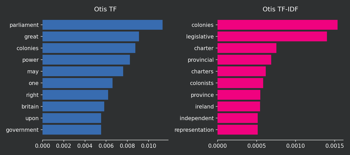

content_copy Copy

TF_IDF_mayhew = thacher_otis_may[["word", "TF-IDF_mayhew"]].sort_values(by = "TF-IDF_mayhew", ascending = False).head(10)
TF_mayhew = thacher_otis_may[["word", "TF_mayhew"]].sort_values(by = "TF_mayhew", ascending = False).head(10)

fig, (ax1, ax2) = plt.subplots(1,2, figsize=(9, 3))

# barplot:
ax1.barh(TF_mayhew["word"], TF_mayhew["TF_mayhew"], color = "#386cb0", edgecolor = "#386cb0")
ax2.barh(TF_IDF_mayhew["word"], TF_IDF_mayhew["TF-IDF_mayhew"], color = "#f0027f", edgecolor = "#f0027f")

# title:
ax1.set_title("Mayhew TF")
ax2.set_title("Mayhew TF-IDF")

for ax in fig.axes:                             # iterate over ax1, ax2, ax3 to: 
    ax.invert_yaxis()                           # invert the y axis; 
    ax.grid(False)                              # eliminate grid;
    ax.title.set_color('white')                 # set title font color to white;
    ax.tick_params(axis='x', colors='white')    # set x axis font color to white;
    ax.tick_params(axis='y', colors='white')    # set y axis font color to white;
    ax.set_facecolor('#2E3031')                 # set ax background color to #2E3031;
    ax.spines["top"].set_visible(False)         # eliminate spines;
    ax.spines["right"].set_visible(False)
    ax.spines["left"].set_visible(False)
    ax.spines['bottom'].set_color('white')

# fig background color:
fig.patch.set_facecolor('#2E3031')
# layout:
fig.tight_layout()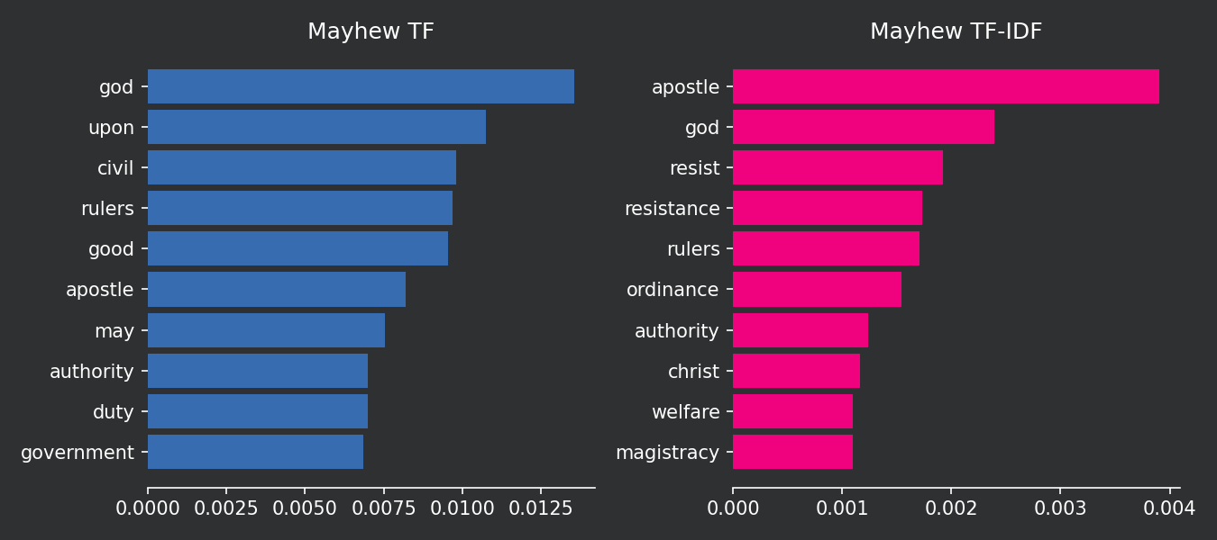

Please note that common words in the corpus, such as “Britain” and “government,” simply do not appear in the top 10 chart because they are present in all three documents. The intuition behind this is that these words are so common in the corpus that they do not provide much useful information. The top 10 words found with TF-IDF have a stronger explanatory power in distinguishing between the three authors. Furthermore, despite being present in two documents, the word “colonies” continues to have a strong TF-IDF score. This is because the word is not present in all three documents, and it is very common in the two documents where it appears.

Conclusions

• TF-IDF depends on two factors: the frequency of a word in a document, and the inverse frequency of the word in the corpus;
• It is possible to calculate TF-IDF scores from scratch in Python, which helps you to understand the logic behind the calculation;
• TF-IDF is a useful tool when you want to identify words that are specific to a particular document.